In 2014, Benjamin Morris published “The Hidden Value of the NBA Steal” on FiveThirtyEight. In his article, Morris argued that both traditional NBA player evaluation and analytics had underrated the value of a player getting steals; he included the eye-catching assertion that “a steal is ‘worth’ as much as nine points.” (More on that later.) With its provocative headline, the article generated a fair amount of discussion in the sports analytics community. Morris ended up writing a four-part response and rebuttal to his critics [1,2,3,4].

It’s a fascinating piece to revisit some seven years past. Knowing where sports analytics went subsequently – increasingly focused on the new frontier of in-game player tracking data – the focus on a basic box-score statistic (steals) feels almost refreshingly quaint.

The rebuttal series by Morris is worth reading as it clarifies the underlying assumptions and intended takeaways of his article. But there’s one issue with the piece left yet undiscussed that is worth diving into — namely that it conflates different types of “value” and as a result falls into the well-known correlation-does-not-imply-causation pitfall, albeit in different garb than usual.

Before laying out my argument, I think it’s worth a raison d’etre for why I’m spending the time writing this and why I’m “picking on” a seven-year-old article written for a somewhat general audience. Here goes: it’s an instructive example of where analytics can go awry in the translation to an audience. There’s nothing wrong methodologically with what Morris has done, only in how it’s been communicated, and even then only subtly. But because of that, the reader may walk away with a very wrong conclusion in mind.

I’ll start by describing Morris’s analysis, identify the overstatement of applicable takeaways, and provide a comparative illustration to baseball. I end by speaking more broadly to why this example should matter to professional analytics teams in any industry, and how to avoid potential missteps.

With that said, let’s dive into the example. Morris’s article relies upon linear regression, so the section below necessarily assumes the reader has some familiarity with regression analysis.

A dive into Morris’s regression analysis

Morris’s assertions are based on a set of coefficients from linear regression. (He shares the methodology but doesn’t share a full regression output table.) The regression is on the player level, and the dependent variable can be described as a measure of player value to his team. (The exact implementation and accuracy of this value metric – see his footnote – isn’t important for our purposes here, and we can just assume that it is correct.) His set of independent variables are basic box score stats: points, rebounds, assists, blocks, steals and turnovers.

Morris pulls the regressions coefficients, sets them relative to the coefficient for a point, and finds that the steal coefficient has a relative magnitude over nine, hence the claim that “a steal is ‘worth’ as much as nine points.”

At this, some readers raised their hands. How can a steal possibly be “worth” nine points? A steal can be seen as the loss of one team’s possession and the gain of an opponent possession. An NBA team averages around one point per possession. Even if the team committing the steal averages, let’s say, two points instead of one because of the fast break, doesn’t the structure of the game then limit the value of a steal to three points?

Morris’s subsequent rebuttal acknowledges he could have clarified the wording – he’s not actually arguing that a steal is worth nine points in the context of an NBA game, simply that for predictive purposes, a marginal steal is weighted nine times more heavily when predicting a player’s impact than a marginal point. If a team’s best player couldn’t play, steals tell us nine times more than points in predicting the impact of his absence on his team’s ability to win the game.

So: Morris is clarifying that the “value” he is referring to is the predictive value of a steal – i.e., how well steals can predict the intrinsic value of a player (his dependent variable). This is the source of confusion: the word “value” is used throughout the piece in at least two different ways – first as predictive value, and second as in-game or intrinsic value.

If the largest misstep were an ambiguous reference to “value,” then there wouldn’t be much to write about. But at a couple points in the piece, the wires get crossed, and the one type of value is mistaken for the other, in ways that invalidate the underlying claims.

Morris writes:

NBA stat geeks have been trying to mash up box score stats for decades. The most famous attempt is John Hollinger’s player efficiency rating [PER], which ostensibly includes steals in its calculation but values them about as much as two-point baskets. […]

Hollinger weights each stat in his formula based on his informed estimation of its intrinsic value. Although this is intuitively neat, empiricists like to test these sorts of things. One way to do it is to compare how teams have performed with and without individual players, using the results to examine what kinds of player statistics most accurately predict the differences. In particular, we’re interested in which player stats best predict whether a team will win or lose more often without him. […]

By this measure [Morris’s analysis], PER vastly undervalues steals. Because steals and baskets seem to be similarly valuable, and there are so many more baskets than steals in a game, it’s hard to see how steals can be all that important. But those steals hold additional value when we predict the impact of the players who get them. A lot more value.

The problem here is that Morris is comparing apples and oranges. Morris clarified that his analysis refers only to the predictive value of steals, but Hollinger’s metric refers to the intrinsic value of steals. These are incomparable. Remember, all Morris’s regression analysis has done is shown an association between steals and overall player value. He has established correlation but not causation; therefore, he can make no claims as to the intrinsic value of the steal. So when Morris asserts that, in comparison to his metric, “PER vastly undervalues steals,” that is unsupported by his methodology.

It’s also worth mentioning the piece’s misleading title — “The Hidden Value of the NBA Steal” — which again falls prey to the double meaning of “value.” In the context of sports analytics, “value” can be assumed to be referring to intrinsic value unless otherwise specified. But the title can only be referring to predicted value, because, again, the regression analysis can make no claims on intrinsic value. I’ll add the caveat that it’s often not authors who write article titles in digital media, but this slippage in the title encourages readers to take away a very wrong conclusion (that steals are underrated in terms of intrinsic value), and I would wager that most did. If we add an appropriate modifier — “The Hidden Predictive Value of the NBA Steal” — the article becomes a lesser pronouncement.

Correlation, causation, and a detour into baseball

Is Morris’s analysis some potential evidence that steals might have more of a game impact than previously assumed, even if he cannot prove that definitively? I’ve heard it said cheekily that “correlation does not imply causation, but correlation is correlated with causation.” Does the same apply here?

No, we can’t assume causality at all, or raise our “priors” on whether steals . It’s helpful here to provide an illustration from baseball that follows the same methodology Morris used but reaches an obviously wrong conclusion.

Let’s specify a regression model — let’s use a team’s total runs scored in a season as our dependent variable, and try to fit this using the independent variables of that team’s total walks, singles, doubles, triples, and home runs.

We get the results below (code here):

                                 OLS Regression Results                                
=======================================================================================
Dep. Variable:                      R   R-squared (uncentered):                   0.998
Model:                            OLS   Adj. R-squared (uncentered):              0.998
Method:                 Least Squares   F-statistic:                          2.098e+04
Date:                Mon, 28 Jun 2021   Prob (F-statistic):                   4.75e-241
Time:                        20:51:29   Log-Likelihood:                         -854.41
No. Observations:                 180   AIC:                                      1719.
Df Residuals:                     175   BIC:                                      1735.
Df Model:                           5                                                  
Covariance Type:            nonrobust                                                  
==============================================================================
                 coef    std err          t      P>|t|      [0.025      0.975]
------------------------------------------------------------------------------
BB             0.1012      0.019      5.203      0.000       0.063       0.140
1B             0.1702      0.025      6.820      0.000       0.121       0.219
2B             0.7697      0.097      7.910      0.000       0.578       0.962
3B             0.5710      0.272      2.097      0.037       0.034       1.109
HR             1.2891      0.075     17.232      0.000       1.141       1.437
==============================================================================
Omnibus:                        4.283   Durbin-Watson:                   2.205
Prob(Omnibus):                  0.117   Jarque-Bera (JB):                4.216
Skew:                          -0.374   Prob(JB):                        0.121
Kurtosis:                       2.953   Cond. No.                     7.61e+15
==============================================================================

Now, let’s follow the same methodology that Morris used, and let’s set all the coefficients relative to one of the other coefficients (in this case, a single). From this we get the following:

We see that a home run is “worth” over seven times as much as a single. (That seems quite high!). Also, we see that a double is “worth” more than a triple! Do these results imply that whenever a team has a runner rounding second base, they should instruct him to hold up there and not advance to third, because doing so increases the chance of scoring?

Of course not. This is just an association. One explanation for these results is that team doubles are more marginally predictive of scoring than team triples because players who hit triples may be smaller and speedier, and hit fewer home runs. But it’s helpful to use the baseball example because the game is structured such that we know that a triple is strictly better than a double. It’s an objective reality check. There would be no issues by simply stating that in the sample used, a team’s number of doubles is observationally associated with run scoring to a greater degree than a team’s number of triples. That appears to be the case. It does not follow that doubles are more intrinsically valuable than triples, even though they have more predictive value for a team’s ability to score runs.

As it turns out, baseball research has well established the intrinsic value of different in-game events (see this article on Fangraphs). To close the loop here, we can use this as an objective comparison to compare how far “off” our naive regression results were vs. the actual values (“linear weights”):

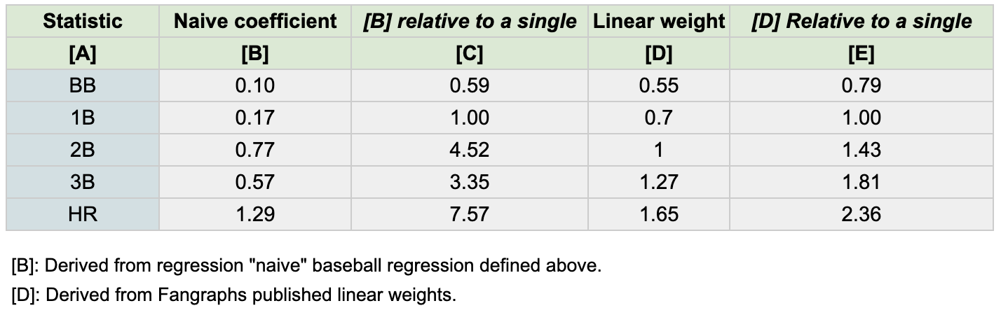
A home run is actually around 2.3x more intrinsically valuable than a single. All this is to show that we cannot interpret the regression results above as implying anything about the intrinsic value of various marginal events in baseball or basketball.

The importance of analytics communication

I mentioned earlier that it’s an instructive example of mistranslation of analytics to an audience. But why is this important – why am I taking the time to write about this?

Throughout my career in product analytics, data science, and quantitative strategy, any project ultimately involves some degree of communicating technical subjects to a less-technical audience. That’s where the impact of my work truly is, and that’s how a data scientist or analytics leader can influence direction and drive change for a business or a product. (If my team’s work isn’t eventually communicated to a less technical audience, it generally hasn’t been successful!). However, assuming a given data analyst is able to present with polish and authority, a less-technical audience may not be able to spot any errors, methodological deficiencies, overstatements, or other sleight of hand (intentional or unintentional). When this occurs, teams and products can internalize the wrong takeaways (as we saw with the basketball analysis above) and make the wrong decisions.

In a broader sense, temptations abound for any Analyst to sacrifice analytical rigor and precision of language. What I if use a different methodology that might exaggerate growth, so my team can hit its stated goals? What if I imply that this new user flow causes a retention boost, when I’m not really sure there’s a causal effect? No one will know but me. Because the Analyst’s outputs can be essentially unauditable by a non-practitioner, we have a principal-agent problem. The principal (company, or colleagues) hires the agent (analyst) to perform a task, but cannot properly measure success because of asymmetric information. How do we solve this, and where are the incentives to not fall prey to this behavior?

A lot of ink can be spilled on this topic, but to summarize: I believe company leadership has to actively seek out and select an Analytics leader committed to enforcing analytical rigor. Analytics and data science teams perform better with some responsibility to a set of professional norms related to meticulousness, clarity of communication, and perhaps even some conception of capital-T Truth. “Honor among analysts’’ is actually the easier part; the harder part, as Morris’s article shows, is making sure that capital-T Truth gets communicated to an audience to the point where it correctly impacts decision-making. And if these truths are “hard truths” in a business context, the audience may be unreceptive. For example, the Analyst will have to argue to a cross-functional group that “we should not ship new product feature ABC because XYZ” when everyone else in the room has their own incentives to want to ship aforementioned new product feature.

So, successful implementation of analytics processes needs to be on the organizational level: it requires that Analysts are protected within a company for telling the hard truths with rigor and clarity – and fighting the fight to make sure their recommendations are followed. And it requires an Analytics leader both who has buy-in to implement “hard truth telling” as standard operating procedures, and has the ability to enforce these norms of rigor within his or her team.